Metrics#
There are a lot of goodness of fit metrics and ways to characterize loss.
Basics#
A model fits the data well when the differences between the observed values and predicted values are small and unbiased
the differences between the
observed valuesandpredicted valuesare calledresidualsas the
goodness of fitincreases, the model is better fitted to the data
Goodness of Fit metrics#
Nomenclature\(y\) = observed values
\(y_i\) = observed value \(i\)
\(\hat y_i\) = predicted value \(i\)
\(\bar y_i\) = average of the observed values \(i\)
\(RSS\) = Residual Sum of Squares = \(\sum_{i=1}^n(y_i-\hat y_i)^2\)
\(TSS\) = Total Sum of Squares = \(\sum_{i=1}^n(y_i-\bar y_i)^2\)
\(DOF_{res}\) = Degrees of Freedom of population variance around mean
\(DOF_{tot}\) = Degrees of Freedom of population variance around model
\(n\) = sample size
\(p\) = total number of explanatory variables (inputs)
R-squared(also known as Coefficient of Determination) is the ratio of the variance that’s explained by the model to the variance that’s explained by a simple mean. It’s usually \(0-1\), though it can be negative if the model is worse at explaining variance than just guessing the mean regardless of inputs. \(R^2\) always increases as more independent variables are added, whether or not those variables are useful predictors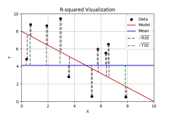
\(\Large R^2=1-\frac{RSS}{TSS}=1-\frac{\sum_{i=1}^n(y_i-\hat y_i)^2}{\sum_{i=1}^n(y_i-\bar y_i)^2}\)
Adjusted R-squaredis a modification of R-squared that penalizes the inclusion of variables that don’t actually contribute to prediction\(\Large \bar R^2=1-\frac{RSS/DOF_{res}}{TSS/DOF_{tot}}=1-(1-R^2)\frac{n-1}{n-p-1}\)
MAE= Mean Absolute Error - same scale as target variable, robust to outliers, difficult to take derivatives of due to absolute value\(MAE = \frac{1}{n} \sum_{i=1}^n|y_i-\hat{y}_i|\)
NMAE= Normalized Mean Absolute Error - normalizes the absolute error by the range of actual values, making it a relative relative metric\(\Large NMAE = \frac{\frac{1}{n}\sum_{i=1}^n{|\hat{y}_i-y_i|}}{\frac{1}{n}\sum_{i=1}^n{|y_i|}} = \frac{MAE(y,\hat{y})}{mean(|y|)}\)
MSE= Mean Squared Error - vulnerable to outliers because the error is squared\(MSE =\frac{1}{n}\sum_{i=1}^n (\hat{y}_i - y_i)^2\)
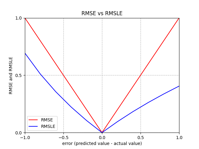
RMSE= Root Mean Squared Error - same training results as using \(MSE\), still vulnerable to outliers, compare with \(MAE\) to see prevalence of outliers\(RMSE = \sqrt{\frac{1}{n}\sum_{i=1}^n (\hat{y}_i - y_i)^2}\)
RMSLE= Root Mean Squared Log Error - logs make it relative metric (ignore scale of data), less vulnerable to outliers than \(RMSE\), asymmetric (larger penalty if \(\hat{y}_i < y_i\) than if \(\hat{y}_i > y_i\))\(RMSLE = \sqrt{\frac{1}{n}\sum_{i=1}^n (\ln{(\hat{y}_i+1)} - \ln{(y_i+1)})^2} =\sqrt{\frac{1}{n}\sum_{i=1}^n (\ln{\frac{\hat{y}_i+1}{y_i+1}})^2}\)
MAPE= Mean Absolute Percentage Error (AVOID LIKE THE PLAGUE) fails if any \(y_i=0\), higher penalty for small \(y_i\), higher penalty for \(\hat{y}_i > y_i\) than \(\hat{y}_i < y_i\)\(MAPE = \frac{1}{n}\sum_{i=1}^{n}{|\frac{y_i-\hat{y}_i}{y_i}|}*100\)
SMAPE= Symmetric Mean Absolute Percentage Error (AVOID) improves somewhat onMAPEbut still controversial, not symmetric, and the equation itself varies by source\(SMAPE = \frac{1}{n}\sum_{i=1}^{n}{\frac{|y_i-\hat{y}_i|}{y_i+\hat{y}_i}}\)
\(BIC\) = Bayesian Information Criterion evaluates goodness of fit \(-2\ln(L)\) while penalizing complexity to avoid overfitting \(k\ln(n)\)
\(BIC = -2\ln(L) + k\ln(n)\)
\(L\) = likelihood of the model given the data
\(k\) = number of parameters in the model
\(AIC\) = Akaike Information Criterion
\(AIC = 2k - 2 \ln(\hat L)\)
\(\hat L\) = maximized value of the likelihood function for the model