Machine Learning Mastery Python Mini Course

• https://machinelearningmastery.com/python-machine-learning-mini-course/

import pickle

import numpy as np
import pandas as pd
import matplotlib.pyplot as plt

from pandas.plotting import scatter_matrix
from sklearn.preprocessing import StandardScaler
from sklearn.model_selection import KFold, cross_val_score, train_test_split
from sklearn.linear_model import LogisticRegression, Ridge
from sklearn.model_selection import GridSearchCV
from sklearn.neighbors import KNeighborsRegressor
from sklearn.ensemble import RandomForestClassifier

Creating DataFrames

Create a simple DataFrame

• then load one in from a CSV at a URL

# Create a DataFrame from a NumPy array
myarray = np.array([[1, 2, 3], [4, 5, 6]])
rownames = ["a", "b"]
colnames = ["one", "two", "three"]
mydataframe = pd.DataFrame(myarray, index=rownames, columns=colnames)
mydataframe

	one	two	three
a	1	2	3
b	4	5	6

Create DataFrame from CSV URL

• this is the Pima Indians “Onset of Diabetes Dataset”

• it’s about the characteristics of the Pima Indians

• the final "class" column is the class of diabetes

• 0 meaning “no diabetes” and 1 meaning “has diabetes”

# Create a Pandas DataFrame from a CSV file from a URL
url = "https://raw.githubusercontent.com/jbrownlee/Datasets/master/pima-indians-diabetes.data.csv"
names = ["preg", "plas", "pres", "skin", "test", "mass", "pedi", "age", "class"]
data = pd.read_csv(url, names=names)
data

	preg	plas	pres	skin	test	mass	pedi	age	class
0	6	148	72	35	0	33.6	0.627	50	1
1	1	85	66	29	0	26.6	0.351	31	0
2	8	183	64	0	0	23.3	0.672	32	1
3	1	89	66	23	94	28.1	0.167	21	0
4	0	137	40	35	168	43.1	2.288	33	1
...	...	...	...	...	...	...	...	...	...
763	10	101	76	48	180	32.9	0.171	63	0
764	2	122	70	27	0	36.8	0.340	27	0
765	5	121	72	23	112	26.2	0.245	30	0
766	1	126	60	0	0	30.1	0.349	47	1
767	1	93	70	31	0	30.4	0.315	23	0

768 rows × 9 columns

Examining the Data

Describe

# Statistical Summary
data.describe()

	preg	plas	pres	skin	test	mass	pedi	age	class
count	768.000000	768.000000	768.000000	768.000000	768.000000	768.000000	768.000000	768.000000	768.000000
mean	3.845052	120.894531	69.105469	20.536458	79.799479	31.992578	0.471876	33.240885	0.348958
std	3.369578	31.972618	19.355807	15.952218	115.244002	7.884160	0.331329	11.760232	0.476951
min	0.000000	0.000000	0.000000	0.000000	0.000000	0.000000	0.078000	21.000000	0.000000
25%	1.000000	99.000000	62.000000	0.000000	0.000000	27.300000	0.243750	24.000000	0.000000
50%	3.000000	117.000000	72.000000	23.000000	30.500000	32.000000	0.372500	29.000000	0.000000
75%	6.000000	140.250000	80.000000	32.000000	127.250000	36.600000	0.626250	41.000000	1.000000
max	17.000000	199.000000	122.000000	99.000000	846.000000	67.100000	2.420000	81.000000	1.000000

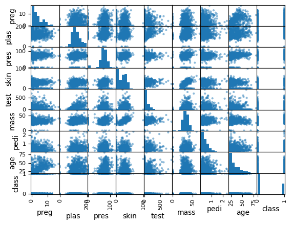
Scatter Plot Matrix

• shows each of the DataFrame columns combined with each other colum

• “pairwise scatterplot”

• where the data combines with itself, you get a histogram showing its distribution

• in the other views, you get points plotted

• so where preg aligns with plas for instance

  • if preg is on the y-axis and plas is on the x-axis

  • it plots the each point’s (x,y) (plas,preg)

# Scatter Plot Matrix
scatter_matrix(data)
plt.show()

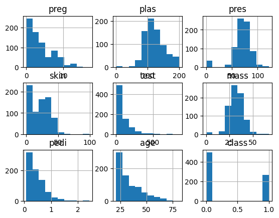
Histogram

• Shows the distribution of each of the columns

• its those midline plots from the scatter plot matrix

data.hist()

array([[<Axes: title={'center': 'preg'}>,
        <Axes: title={'center': 'plas'}>,
        <Axes: title={'center': 'pres'}>],
       [<Axes: title={'center': 'skin'}>,
        <Axes: title={'center': 'test'}>,
        <Axes: title={'center': 'mass'}>],
       [<Axes: title={'center': 'pedi'}>,
        <Axes: title={'center': 'age'}>,
        <Axes: title={'center': 'class'}>]], dtype=object)

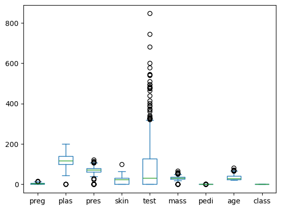
Box Plot

• shows all of the distributions of the points on the same axes

• wonder why test has SO many outliers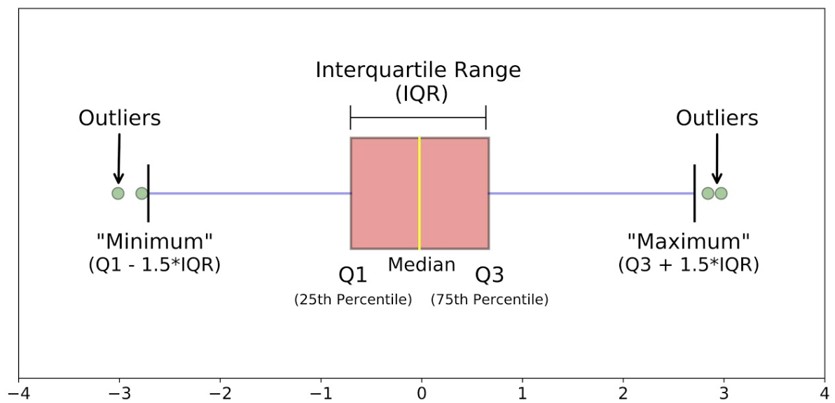

• 

data.plot(kind="box")

<Axes: >

Pre-Processing Data

• Standardize numerical data (set mean to 0, standard deviation of 1) with scale and center options

• Normalize Numerical Data (min=1, max=1) using range option

• Advanced options like Binarizing

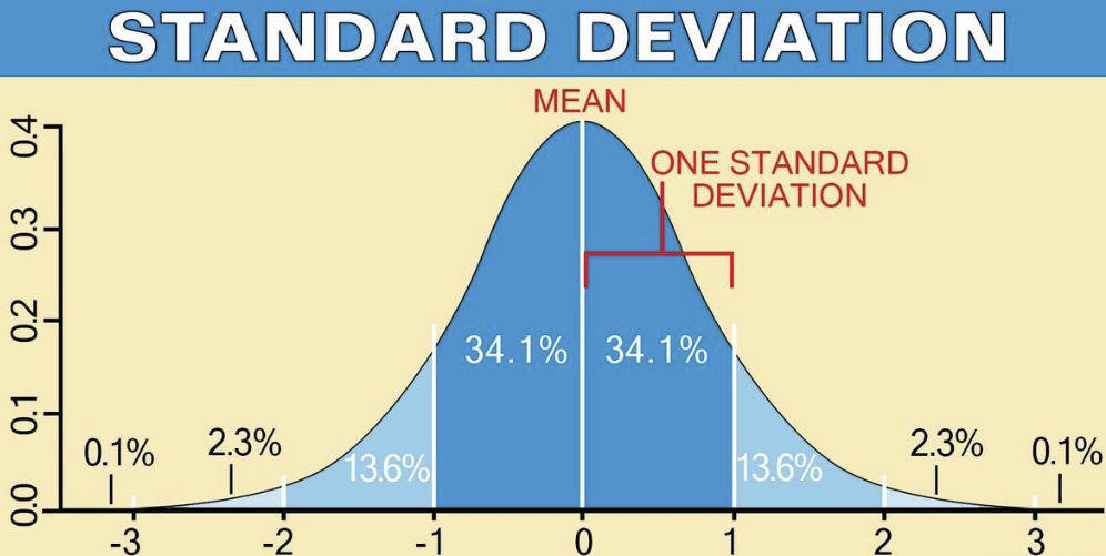
Standardize (Scale and Center)

• mean = 0 , standard deviation = 1

• so basically this?

• hmm. Looks like image attachments don’t play well with html image links, though Stack Overflow seems to think it should work?

• 

# Standardize data (0 mean, 1 stdev)
array = data.values
# separate array into input and output components
X = array[:, 0:8]  # all rows, columns 0-7 (it's not inclusive of the end)
Y = array[:, 8]  # all rows, column 8
scaler = StandardScaler().fit(X)
rescaledX = scaler.transform(X)
# set NumPy to print numbers with up to 3 decimal places
np.set_printoptions(precision=3)
# show rows 0-4 of the rescaled data
# sreveals that mean is now 1, the standard deviation of all of these is 1
rescaledX[0:5, :]

array([[ 0.64 ,  0.848,  0.15 ,  0.907, -0.693,  0.204,  0.468,  1.426],
       [-0.845, -1.123, -0.161,  0.531, -0.693, -0.684, -0.365, -0.191],
       [ 1.234,  1.944, -0.264, -1.288, -0.693, -1.103,  0.604, -0.106],
       [-0.845, -0.998, -0.161,  0.155,  0.123, -0.494, -0.921, -1.042],
       [-1.142,  0.504, -1.505,  0.907,  0.766,  1.41 ,  5.485, -0.02 ]])

Resampling

• training dataset - data used to train the machine learning algorithm

• you can’t use data that was used to train the algorithm to estimate the accuracy of the model for predicting on new data

• Resampling - split the training dataset into subsets. Use some data to train, hold some back to check

K-Fold Cross Validation

• split the dataset into 10 parts (9 to train, 1 to test)

• shuffle the order so the splits are randomized

• set a random seed so that it’s reproducible

# create a K-fold cross-validator to split the dataset
kfold = KFold(n_splits=10, random_state=7, shuffle=True)
# create a logistic regression model
model = LogisticRegression(solver="liblinear")
# train the logistic regresssion model, use the kfold to split the data up
results = cross_val_score(model, X, Y, cv=kfold)
# print the accuracy and standard deviation of the model
print(f"Accuracy: {results.mean() * 100.0:.3f}")
print(f"Standard Deviation: {results.std() * 100.0:.3f}")

Accuracy: 77.086
Standard Deviation: 5.091

Evaluation Metrics

• many metrics can be used to evaluate how well an algorithm predicts on a dataset

Logloss

results = cross_val_score(model, X, Y, cv=kfold, scoring="neg_log_loss")
print(f"Logloss: {results.mean():.3f}")
print(f"Logloss Standard Deviation: {results.std():.3f}")

Logloss: -0.494
Logloss Standard Deviation: 0.042

• the following headings were mentioned in the chapter on the site

• but there’s no further explanation or accompanying code

• I guess I’m supposed to be figuring those out on my own?

• there are probably equivalent ones on each other chapter that I missed

Confusion Matrix

Classification Report

RMSE and R-Squared

Spot-Check Algorithms

• there are a LOT of machine learning algorithms

• figuring out which one performs best on your data will require some level of trial-and-error

• he refers to this as spot-checking algorithms

Linear Algorithms

• linear regression

• logistic regression

• linear discriminate analysis

Non-Linear Algorithms

• KNN - K-Nearest Neighbors

• SVM - Support Vector Machine

• CART - Classification and Regression Trees

• start out with the Boston House Price dataset

# Prepare data from the Boston House Price dataset
url = "https://raw.githubusercontent.com/jbrownlee/Datasets/master/housing.data"
names = [
    "CRIM",
    "ZN",
    "INDUS",
    "CHAS",
    "NOX",
    "RM",
    "AGE",
    "DIS",
    "RAD",
    "TAX",
    "PTRATIO",
    "B",
    "LSTAT",
    "MEDV",
]
dataframe = pd.read_csv(url, delim_whitespace=True, names=names)
array = dataframe.values
X = array[:, 0:13]
Y = array[:, 13]
kfold = KFold(n_splits=10, random_state=7, shuffle=True)

/tmp/ipykernel_2243/190392337.py:19: FutureWarning: The 'delim_whitespace' keyword in pd.read_csv is deprecated and will be removed in a future version. Use ``sep='\s+'`` instead
  dataframe = pd.read_csv(url, delim_whitespace=True, names=names)

# Train a K-Nearest Neighbors model on the Boston House Price dataset
model = KNeighborsRegressor()
scoring = "neg_mean_squared_error"
results = cross_val_score(model, X, Y, cv=kfold, scoring=scoring)
print(f"Negative MSE: {results.mean():<.3f}\nStd Dev: {results.std():<.3f}")

Negative MSE: -38.852
Std Dev: 14.661

Ensemble Algorithms

• random forest

• stochastic gradient boosting

Model Comparison and Selection

• after spot checking a few algorithms, must compare performance

  • Compare linear algorithms to each other on a dataset.

  • Compare nonlinear algorithms to each other on a dataset.

  • Compare different configurations of the same algorithm to each other.

  • Create plots of the results comparing algorithms.

• this example trains a couple of algorithms on the PIMA diabetes dataset and compares their accuracy

# Compare Algorithms
from pandas import read_csv
from sklearn.model_selection import KFold
from sklearn.model_selection import cross_val_score
from sklearn.linear_model import LogisticRegression
from sklearn.discriminant_analysis import LinearDiscriminantAnalysis

# load dataset
url = "https://raw.githubusercontent.com/jbrownlee/Datasets/master/pima-indians-diabetes.data.csv"
names = ["preg", "plas", "pres", "skin", "test", "mass", "pedi", "age", "class"]
dataframe = read_csv(url, names=names)
array = dataframe.values
X = array[:, 0:8]
Y = array[:, 8]

# prepare models
models = [
    ("Logistic Regression", LogisticRegression(solver="liblinear")),
    ("Linear Discriminant Analysis", LinearDiscriminantAnalysis()),
]
# evaluate each model in turn
scoring = "accuracy"
kfold = KFold(n_splits=10, random_state=7, shuffle=True)
print("Accuracy and Standard Deviation for each model:")
# train and evaluate each model in turn
for name, model in models:
    cv_results = cross_val_score(model, X, Y, cv=kfold, scoring=scoring)
    print(f"{name}: {cv_results.mean():.3f} ({cv_results.std():.3f})")

Accuracy and Standard Deviation for each model:

Logistic Regression: 0.771 (0.051)
Linear Discriminant Analysis: 0.767 (0.048)

Improving Model Accuracy

Parameter Tuning

• once you’ve identified an algorithm or two that works well, tune them to improve their performance

• for example, by tuning the parameters to your specific dataset

• this sounds like hyperparameter tuning

• scikit-learn has a couple of way to search for good parameters

  • grid search (that you specify)

  • random search

• the below example uses a grid search to set the parameters of a linear Ridge model trained on the Pima Indians Diabetes Dataset

  • grid search is expensive since it trains and checks every combination

# Grid Search for Algorithm Tuning
# create an array of alpha parameters to check
alphas_list = [1, 0.1, 0.01, 0.001, 0.0001, 0]
alphas = np.array(alphas_list)
# create a parameter grid dictionary
# where the key is 'alpha' and the value is the array
# this format allows you to search a grid of multiple parameters
param_grid = dict(alpha=alphas)
# create a ridge regression model
model = Ridge()
# create a grid search object to check all values of alpha
# this time, use 3-fold cross validation
grid = GridSearchCV(estimator=model, param_grid=param_grid, cv=3)
# train the model for each
grid.fit(X, Y)
# announce the best
# best score of 0.280? that's pretty low
print(f"alphas checked: {alphas_list}")
print(f"best score: {grid.best_score_:.3f}")
print(f"best alpha: {grid.best_estimator_.alpha:.3f}")

alphas checked: [1, 0.1, 0.01, 0.001, 0.0001, 0]
best score: 0.280
best alpha: 1.000

Ensemble Predictions

• Practice bagging ensembles with

  • random forest and extra trees algorithms

  • gradient boosting machine and AdaBoost algorithms.

• Practice voting ensembles by

  • combining the predictions from multiple models together

• the following code demonstrates using the Random Forest algorithm on the Pima Indians Diabetes Onset dataset

  • Random Forest is a “bagged ensemble of decision trees”

# make a KFold cross-validator to split it up
kfold = KFold(n_splits=10, random_state=7, shuffle=True)
# set parameters and create the Random Forest model
num_trees = 100
max_features = 3
model = RandomForestClassifier(n_estimators=num_trees, max_features=max_features)
# train and score the model (takes longer than the lineaer ones)
results = cross_val_score(model, X, Y, cv=kfold)
print(f"Random Forest Accuracy: {results.mean():.3f}")

Random Forest Accuracy: 0.773

Finalize and Save

• once you’ve got a tuned, well-performing model, finalize and save it

• practice making predictions on new (unseen) data

• save the model to file

  • I seem to recall there was a format other than pickle that was better for machine learning models

• load it from file and score it

# split the dataset into train and test sets
# this time do it manually since we're training and scoring separately
X_train, X_test, Y_train, Y_test = train_test_split(
    X,  # unsplit inputs
    Y,  # unsplit outputs
    test_size=0.33,  # hold back 1/3 of the data for testing
    random_state=7,  # set a seed for reproducibility
)

# Fit the Logistic Regression model on the training data (2/3rds of the data)
model = LogisticRegression(solver="liblinear")
model.fit(X_train, Y_train)

# save the model to disk as a compressed "pickle" file
filename = "finalized_model.sav"
pickle.dump(model, open(filename, "wb"))

# some time later...

# load the model from disk
loaded_model = pickle.load(open(filename, "rb"))

# check how well the loaded model performs on the test set
result = loaded_model.score(X_test, Y_test)
print(f"Logistic Regression Accuracy: {result:.3f}")

Logistic Regression Accuracy: 0.756